Feature Extraction
Vision. Yeah, that magic thing we throw OpenCV at every year, unfailingly producing beautiful code destined to die having never run on the robot. In FRC, the goal of ‘simple’ vision is rather, well, simple: rectangles of retroreflective tape are attached to a goal and, by tracking the position of those pieces of tape and their relative size in the image, you can figure out where you are relative to the goal. The specifics of this aren’t too complicated, but to avoid another 1000-word-blog-post, I’ll refrain from going into them. So let’s instead generalize. ‘Computer Vision’ is a lot of things, among them such stuff as image processing, pattern recognition, image analysis, and so on. The topic we’re going over today falls squarely into a subcategory of the first listed there: Feature Extraction, one of the many components of image processing.
When you have some sort of image, there are many ways to analyze it: you can look for color balance, look for patterns, analyze some mathmatical representation, whatever. What’s often the most useful, however, is being able to extract simple (or complex) objects from the image, rendering them from a series of pixels on a map to a clear, discrete mathmatical representation. Humans do this every day: you look at your walll, you see a rectangular door, you see a circular photograph, you see a triangular… potato chip or whatever. Now, feature extraction doesn’t have to revolve around geometric shapes, it’s just that that’s one of the more common (and simpler) applications of the field. You’re taking something complicated, something dense and unreadable, and rendering it down into discrete, easily processed features of whatever form you may wish.
Lines
Yeah, lines. That’s the feature we’re looking at today. If you expected some fancy facial recognition setup… well, give me a few more blogposts and we’ll see where we get. Now, it turns out that being able to identify lines is rather important, especially given that most other geometric objects you’ll commonly encounter are composed of well… lines. I hope I don’t have to explain how that works with a rectangle or whatever. And it’s harder to accomplish this recognition than you may expect, for a couple of reasons, actually. Firstly, images you’re picking up aren’t going to be clean and crisp; you’ll have noise, distortions, and just flaws that make it impossible to do something like iterate across the image with a straight line and find what matches. Secondly, lines in the real world aren’t usually actually linear: whether it be perspective or just physical imperfection, things tend to be a bit… curvy when you look at them in real life. And finally, well, there are a lot of them. Any one point can have infinite lines going through it: an image can be criss-crossed by lines of any size, direction, and offset, meaning that if you’re going to try and brute force it, you’ll be having a very bad time very quickly. So we don’t do that.
Parameter Space
Instead, let’s look at this mathematically. First of all, what are lines composed of? Points. And if a line exists between three points, what does that mean about the lines you can draw through each point? Well, there’ll be one line you draw through each of the points that’ll be, well, the same line. Y’now, the one that’s… being drawn through each point. If it seems stupidly simple, well, it is, but it’ll become important in a moment. So, if we know points compose lines, why not analyze this problem from the perspective of points, rather than lines? Points are simple: (x,y). Maybe a z if you hate freedom, but we’ll be sticking with 2-d. Lines travel through an entire image, crossing every which way, wheras a point is nicely, concretely defined! Great. So lets redefine the problem: instead of finding lines in an image, find out whether a series of points lie on the same line. If you can do this for all sets of points in an image, well, you’ve got your lines! So how did we figure out if multiple points were on the same line? Well, we took each point, drew every single line that went through said point, and tried to figure out if any of these lines were the same line that goes through another point.
Now, this is something we can do: take some arbitrarily small angle, take a starting line, and slowly cycle it around the point in increments of that angle, and you’ll more or less have ‘every single’ line that can go through that pixel- at least in the context of a by-nature discrete pixel-based image. Well, if we want to log each line that goes through a pixel and compare them to some other infinite-set-of-lines-going-through-another-point, we’ll need some way of defining a line without, well, drawing it. If you cast your mind back to the dark days of Algebra 1, you might remember a little thing they liked to call slope-intercept-form. Y’now, define a line in terms of y = mx + b, where ‘m’ is the slope of the line and ‘b’ is how high up on the y axis it’ll hit when x = 0. So we take all the lines that go through a point and represent them in Slope-Intercept form via ordered pairs: (Slope, Intercept). Doing this forms something called a “Parameter Space”: mapping a series of mathematical objects into some other, equally detailed, representation. Nice thing about this is that we could graph these ordered pairs on a cartesian axis… or can we? Well, in general, yes, you can 100% graph a parameter space, as long as the input is bounded of course. Well, what happens when you have a vertical line, or something near it? Oh right, x = infinity… sucks, can’t graph that. So switch them: (Intercept, Slope). Well… it’s better, but now you have discontinuities in the graph where it flips to infinity and then back to negative infinity… ew. So we need some new method of representing lines, something that is quick, simple, and doesn’t tend towards infinity when the line does something weird.
Hough Space
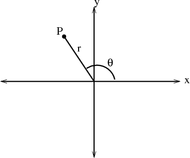
Well, the nice thing about science is that you don’t have to do everything yourself: other people, many of them much smarter than ourselves, have done the heavy lifting for us! So, Hough Space! Those of you who’ve taken Precalculus will know about the idea of Polar Geometry, but for the rest of you, I’ll skim over it here. In cartesian geometry, you define all points by their distance along two axes, represented as a pair (x,y). In polar space, you still use a single ordered pair to represent any point, but you do it… differently. Instead of finding distance along two axes, you draw a line between the point and the origin (the ‘pole’) and extract two values: r and θ (theta). ‘r’ represents the length of the line you’ve drawn: how far away the point is from the pole. θ represents the angle between that line and the ‘x-axis’, or technically just a ‘0-position’ line lying in the same position the ‘x-axis’ would in cartesian coordinates. The angle is measured counterclockwise, as seen below:
So… now we can represent points in a different way. Cool, I guess, but not very useful for representing lines: or is it? What if we could define some point on the line that defines the entire line? Well, technically this is impossible: you need two points to define a line and there’s no way around it; but, when you think about it, we already have a point, don’t we? The origin!
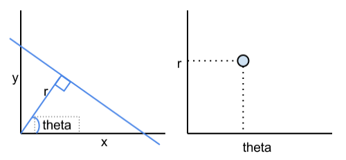
For any line ‘l1’ , we can define it in Hough Space by drawing a second line ‘l2’ starting at the origin and ending up perpendicular to l1. The line l1 is then defined in Hough Space by the ordered pair (r, θ) that represents the intersection of l2 and l1!
So now we can take any point in an image, and as long as we have a defined ‘origin’, we can list every single useful line that passes through said point, without anything going to infinity! And not only does the graph behave in a bounded manner, it actually forms regular, recognizable shapes!
Spooky Scary Sinusoids
What shapes, you might ask? Well, if it isn’t obvious by the repeated articular-memes presented so far, graphing the set of all lines that pass through any given point in a cartesian coordinate system where x = ‘r’, y = ‘θ’ will give you a sinusoid!
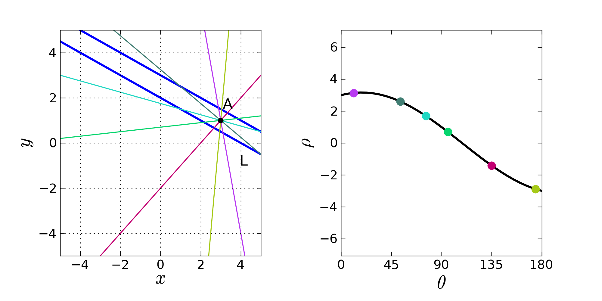
So now, how do we actually find if multiple points lie along the same line? Well, let’s look at what each sinusoid really means. In the end, each of these sinusoids is a representation of a point, but in a really descriptive way: each point on the sinusoid represents a line going through the original point we’ve now transcribed. So if you have multiple ‘original points’, what’ll it look like if they lie along a single line? Well, that means that some line, represented by a single (r, θ), passes through each point: in Hough Space, this means that both points sinusoids will have to contain the cartesian coordinate corresponding to that (r, θ): they intersect! If you have some thousand points, you can figure out which ones lie on the same line by just drawing them in Hough Space and seeing where the most sinusoids intersect: these regions of ‘high activity’ represent lines that are most likely to actually exist in the original image!
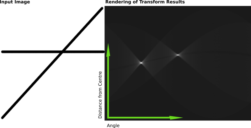
In reality, you’re probably going to have a very large set of points, so the result will be a little less obvious. How, you might ask, do we determine how many points really mean a line is there? You could surely have three points that just happen to be colinear, even if there isn’t a line there in the image: why not 4, 5, or 100? Well, in the end, that’s where the human part of vision processing comes in: you have to define threshold and see how they work! Still, it’s not actually that hard: even in more ‘real world’ situations, it tends to be pretty obvious where the lines are: in the following image, the two white ‘blobs’ correspond to the two lines on the left, pretty obviously.